In this post, I am going to do a quick recap of what a Proximal Operator is -I can see you cringe, Guillaume! -, because there are very useful, especially in large scaled problems, but also not always easy to comprehend.
I highly recommend the classes from Wotao Yin and Lieven Vandenberghe at UCLA on this topic; they are very didactic, and mathematically rigorous. I will heavily rely on their notations.
But I was doing fine with the gradient descent!
Yes, gradient descent is a wonderful optimization tool... if you know for sure the function you want to optimize is smooth. But proximal algorithms are also along the same lines as the gradient descent. Let me explain.
Let's first go back to the case where the function \(f : \mathbb{R}^n \rightarrow \mathbb{R}^n\) you want to optimize is smooth and convex. Then the gradient update can be written, \(\forall i \in \) as: $$ \begin{align} x_{k+1} = x_{k} - \lambda \nabla f (x_{k}) \end{align} $$ The idea between gradient descent is to locally approximate the Taylor expansion of \(f\) at \(x_{k}\) and adding a smoothing term: $$ \begin{align} \tilde{f} (x) = x_{k} + \langle \nabla f (x_k), x - x_k \rangle + \frac{1}{2\lambda} \| x - x_k \|^2 \end{align} $$ And find the point \(x^* \) that minimizes this expression. So we can compute the gradient of \(\tilde{f}\) and equate it to zero. The solution for \(x\) is the following: $$ \begin{align} x^{*} = x_{k} - \lambda \nabla f (x_{k}) \end{align} $$ In an iterative scheme, we can find the gradient descent update. For these of you who are familiar with it, we can recognize a Backward Euler equation here: \(x(t+1) = x(t) - \Delta t f(x(t+1))\). This take the form of a differential equation, that can be solved through the following iterations:
- \(u(t+1) = u^*, \text{with} \ u^* \text{solution of} \ u^* = \nabla f(x(t) - \Delta t u^*)\)
- \(x(t+1) = x(t) - \Delta t u(t+1)\)
So now, if we recall the definition of a proximal operator: $$ \begin{align} prox_{\tau f} (x) = \arg \min_y (f(y) + \frac{1}{2 \tau} \|x - y\|^2) \end{align} $$ Let's first and foremost recall the existence and unicity of such a minimizer for the corresponding optimization problem to minimize. \(f\) is convex by hypothesis, and the second term is strictly convex; which makes the sum of the two functions a strictly convex one, which proves the unique minimum exists. Then the optimality condition is: $$ \begin{align} x^* = y - \tau \nabla f (x^*) \end{align} $$ So the proximal operator returns the optimal \(x^*\) to the first step mentioned above; and \(\nabla f(prox_{\tau f} (y))\), returns our \(u^*\) in our second step mentioned above. So applying a proximal operator is like doing an implicit gradient step!
It also work when \(g\) is non-smooth
Let's say one needs to minimize \(x \mapsto f(x) + g(x) \), both functions convex, \(f\) differentiable, and \(g\) non smooth. The problem is now considered "splitted". The iterative update that we mentioned above is the following: \(x_k = prox_{\lambda, f} (x_{k-1} - \lambda_k \nabla g (x_{k-1}))\). \(prox_{\lambda, f}\) is considered a "backward pass" and the \(x_{k-1} - \lambda_k \nabla g (x_{k-1}))\) is considered a "forward pass". But where did the forward pass term come from? Well, we know that: $$ \begin{aligned} 0 \in \nabla f (x^*) +\partial g (x^*) & \Leftrightarrow & 0 \in \lambda \nabla f (x^*) + \lambda \partial g (x^*) \\ & \Leftrightarrow & 0 \in \lambda \nabla f (x^*) + x^* - x^* + \partial g (x^*) \\ & \Leftrightarrow & (I - \lambda \nabla f)(x^*) \in (I + \lambda \partial g)(x^*)\\ & \Leftrightarrow & (I - \lambda \nabla f)(x^*) \in (I + \lambda \partial g)(x^*)\\ & \Leftrightarrow &(I + \lambda \partial g)^{-1} (I - \lambda \nabla f) (x^*) = x^* \end{aligned} $$ So we can definitely recognize the forward-backward formulation. We can also see that a minimizer of our problem is the fixed point of the operator: \((I + \lambda \partial g)^{-1} (I - \lambda \nabla f)\).
This algorithm is known as "Forward-Backward Splitting" or "Proximal Gradient" and the convergence looks like this in 1D:
Now let's see this forward-backward mechanism through duality. Our optimization problem: $$ \begin{aligned} & \underset{x}{\text{minimize}} & & f(x) + g(x) \end{aligned} $$ is equivalent to the following optimization problem: $$ \begin{aligned} & \underset{x, y}{\text{minimize}} & & f(x) + g(y) \\ & \text{subject to} & & x-y = 0. \end{aligned} $$ Then, let's pose \(z = x-y \) and the augmented Lagrangian (Lagrangian + quadratic penalty) is the following, by definition: $$ \begin{align} L(x, y, z)= f(x) + g(y) + \frac{1}{2\lambda} z^T (x-y) + \frac{1}{2 \lambda} \|x-y\|_2^2 \end{align} $$ which can be rewritten (through calculations with the scalar product associated with the chosen norm - here the Euclidean norm): $$ \begin{align} L(x, y, z)= f(x) + g(y) + \frac{1}{2\lambda} \|x - y + z \| - \frac{1}{2 \lambda} \|z\|_2^2 \end{align} $$ By freezing alternatively \( (y, z) \) and minimizing \(L\) wrt x, then freezing alternatively \( (x, z) \) and minimizing \(L\) wrt y, and then updating \(z_k = x_k - y_k\), we alternatively compute the proximal operators related to \(f\) and \(g\) on the gradient of the augmented Lagrangian.
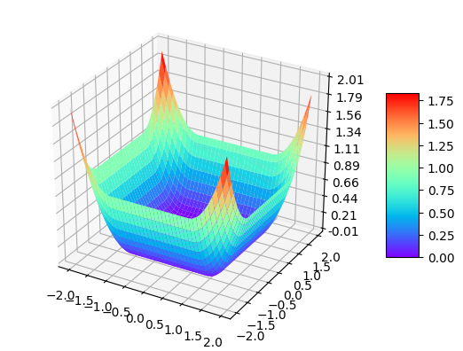
Out of curiosity, here is a plot of the shape of the proximal operator for the \(L_1\) norm:
A third way to comprehend the proximal operators is through the Moreau Envelope. We have seen in a previous post that when a function is non-smooth, but convex and closed, its Moreau Envelope \(\mathcal{M}_{\lambda, f}\) is a smooth function and shares the same global minimizer as \(f\). $$ \begin{align} \mathcal{M}_{\lambda, f} (x) = \inf_{y} (f(y) + \frac{1}{2 \lambda} \|y - x\|^2) \end{align} $$ \(y\) is optimal for \(y^* = prox_{\lambda f} (x)\) so: $$ \begin{align} \mathcal{M}_{\lambda, f} (x) = f(prox_{\lambda f} (x)) + \frac{1}{2 \lambda} \|prox_{\lambda f} (x) - x\|^2 \end{align} $$ So \(\mathcal{M}_{\lambda, f}\) is convex and \(dom (\mathcal{M}_{\lambda, f}) = \mathbb{R}^n\). On top of that, \(\mathcal{M}_{\lambda, f}\) is \(\mathcal{C}^1\). The relation between the proximal operator and the Moreau Envelope of a function \(f\) is as follows: $$ \nabla \mathcal{M}_{\lambda, f} (x) = \frac{1}{\lambda} (x - prox_{\lambda f} (x)) $$ And \(prox_{\lambda f}\) is well defined if \(f\) sub-differentiable.
It is also worth noting that the Moreau Envelope is linked to the augmented Lagrangian through duality, through a clever change of variable.
When should I choose a proximal algorithm ?
Well the scope of proximal algorithms is quite large: it includes smooth and non-smooth functions to minimize, for constrained or unconstrained problems. It can also yield some very nice parallel / distributed implementations, and hence handle large size problems if \(f\) and \(g\) are separable into \( f = \sum_{i} f_i \) and \( g = \sum_{j} g_j \); the updates for each element in the sum can be processed independently and hence in parallel.
Its main constraint (;)) though, is that it works for structured problems only; which is why you can see such methods applied in the computer vision community, as well as the sound / signal processing community.
You can leave comments down here, or contact me through the contact form of this blog if you have questions or remarks on this post!