In this post, we are going to discuss a very powerful -mathematically as well as pragmatically- optimization framework; the First Order Primal Dual Convex Optimization Technique. This involves a few definitions that may not look friendly at first, but the framework is in fact relatively understandable. The framework has successfully been applied to image denoizing and image inpainting, and is really worthy of spending some time to comprehend it.
We will remind a couple of definitions that are useful in this framework, but you can find many more details, definitions, theorems and proofs in "Convex Analysis" by Hiriart-Urruty and Lemarchal, "Convex Optimization" by Boyd and Vandenberghe or "Optimization. Applications in image processing." by Nikolova (the latter two are available freely in pdf format).
We are going to consider here a general problem of the form: $$ \begin{align} & \underset{x}{\text{minimize}} & & \sum_{i \in \Omega} M_i(x_i) + R(Lx) \end{align} $$ with:
- \(M_i\) a lower semi continuous function
- \(R\) a lower semi continuous function
- \(L\) a continuous linear operator
I strongly suggest this excellent paper from A. Chambolle : An introduction to Total Variation for Image Analysis, since it is the paper we are going to base this blog post on.
Soooo.... Why is this useful, again?
Let's say you need to denoise an image for instance. In the Total Variation context, you can write image denoising as the following optimization problem: $$ \begin{align*} & \underset{x}{\text{minimize}} & & \left\| \nabla x\right\|_{1} + \frac{\lambda}{2} \left\| x - f \right\|^2_2 \end{align*} $$ where:
- \(x \in X\) is the sought solution,
- \(f \in X\) is the noisy input image,
- \(\lambda \in \mathbb{R} \) is a parameter to define the trade of between regularization and data fitting,
- \(\left\| \nabla x \right\|_{1}\) represents the discretized version of the isotropic total variation of the function \(x\).
The Total Variation (TV) framework also allows for a nice formulation of the motion estimation problem: $$\begin{align} \min \limits_{x\in \mathcal{X}, v \in \mathcal{Y}} \left\| \nabla u \right\|_{1} + \left\| \nabla v \right\|_{1} + \lambda \left\| \rho (u, v) \right\|_{1} \end{align}$$ where:
- \((u, v)\) are the apparent motion vectors,
- \(\left\| \nabla u \right\|_{1} + \left\| \nabla v \right\|_{1}\) is the total variation of the apparent motion field,
- \(\left\| \rho (u, v) \right\|_{1} = I_{t} + (\nabla I)^T (v - v_0) + \beta u \) is the linearization of the assumption that the intensities of the pixels stay constant over time, known as the Optical Flow Constraint, plus a term that takes into account a drift in the value of pixels over time,
- \(\lambda \in \mathbb{R} \) is a parameter to define the trade of between regularization and data fitting,
- \(\left\| \nabla u \right\|_{1}\) represents the discretized version of the isotropic total variation of the function \(u\).
This same TV framework can also be used for inpainting: $$\begin{align} \min \limits_{x\in \mathcal{X}} \left\| \Phi u \right\|_{1} + \frac{\lambda}{2} \left\| u-g \right\|_{2}^2 \end{align}$$ where:
- \(u\) is the sought solution,
- \(g \in X\) is the noisy input image,
- \(\Phi\) is a linear operator, which can be \(\nabla\) or the Fast Discrete Curvelet Transform for instance,
- \(\left\| \Phi u \right\|_{1}\) is,
- \(\left\| u-g \right\|_{2}^2\) is the linearization of the assumption that the intensities of the pixels stay constant over time,
- \(\lambda \in \mathbb{R} \) is a parameter to define the trade of between regularization and data fitting.
The aim of the inpainting model is to find a sparse representation of the image \(u\) in the domain of \(\Phi\). This is achieved through minimizing the L1 norm.
Useful definitions
Let's first define a couple of concepts that will be useful to us. A function \(f\)on a normed real vector space \(V\) is proper if \(f: V \rightarrow ]-\infty , \infty] \) and if it is not identically equal to \(+\infty \).
A function \(f\) on a normed real vector space \(V\) is coercive if \(\lim_{\left\|u \right\| \rightarrow + \infty} f(u) = + \infty\).
Most of the functions we will consider here will be lower semi-continuous. This means that a function \(f\) on a real topological space \(\mathcal{X}\), \(f: V \rightarrow ]-\infty , \infty] \) is lower semi-continuous (l.s.c.) if \( \forall \lambda \in \mathbb{R}\), the set \( {u \in V: f(u) \leq \lambda}\) is closed in V.
This property is quite important, as we will see in the following theorem: Let \(U\) be non-empty and closed, and \( f : \mathbb{R}^n \rightarrow \mathbb{R}\) be l.s.c.and proper. If \(U\) is not bounded, we also suppose that f is coercive. Then: \(\exists \hat{u} \in U s.t. f(\hat{u}) = inf_{u \in U} f(u)\).
This is actually very important; it means that if \(f\) has all the aforementioned properties, it takes a minimum value on any set \(U\) non-empty and closed.
We will suppose here that you are familiar with the concept of convex functions and sets.
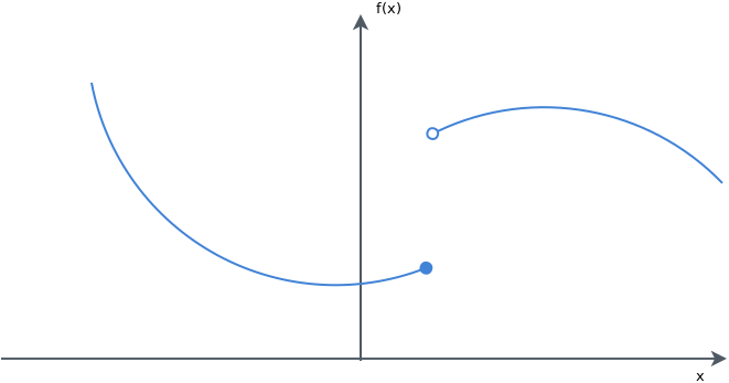
The Moreau Envelope
In our image denoising or inpainting context, the function to optimize may not be smooth, and this complicates the task of minimizing/optimizing the objective function. In order to alleviate this difficulty, a brilliant idea has been introduced in "Proximité et dualité dans un espace hilbertien" by Moreau. Given a proper lsc convex function \( F : \mathcal{X} \leftarrow \mathbb{R} \), the Moreau envelope constructs a smoothed version of function \(F\) where the degree of smoothing is controlled by a parameter \(\tau\). The Moreau envelope is defined as the unique solution of the optimization problem: $$ \begin{align} \mathcal{M}_{F, \tau} (\tilde{x}) = \min \limits_{x \in \mathcal{X}} F(x) + \frac{1}{2 \tau} \left\| x - \tilde{x} \right\|_2^2 \end{align} $$
We note that this problem is smooth and it admits a unique minimizer due to the added smoothing \(\mathcal{l}_2\) norm term.
This being said, just because a problem is strictly convex doesn't mean it is easy to solve. So basically, if \( F \) is hard to optimize, the Moreau envelope is likely difficult to compute. Nonetheless, there exist some functions whose Moreau envelope computation yields a closed form.
We can associate to this function the following operator: $$ \begin{align} prox_{F, \tau} (\tilde{x}) = \arg \min \limits_{x \in \mathcal{X}} F(x) + \frac{1}{2 \tau} \left\| x - \tilde{x} \right\|_2^2 \end{align} $$ that returns the unique minimizer of the Moreau envelope. This operator is called the proximal operator.
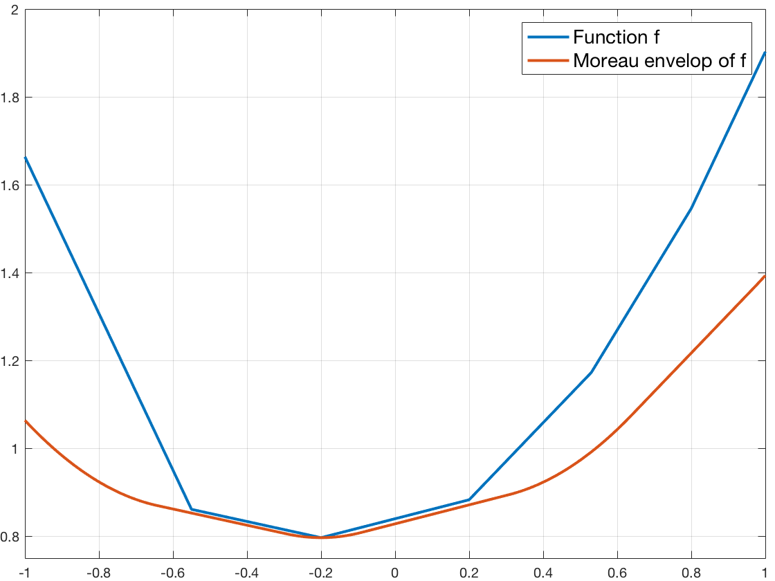
Here is a figure to illustrate what the Moreau envelope is on a non-smooth function, with \(\tau=1\) :
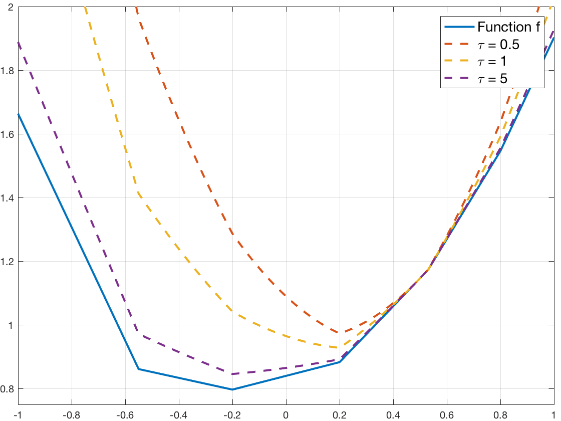
Here is figure to illustrate the influence of the \(\tau\) parameter. We draw the function \(F\) and the functions \(x \mapsto F(x) + \frac{1}{2\tau} \left\| x - \tilde{x} \right\|_2^2 \), with \(\tilde{x}\) fixed at 0.5, with various \(\tau\) values:
The Fenchel Transform
Another difficulty of this optimization problem is the coupling of variables \(x_i\) due to the linear operator \(L\) and the function \(R\). Combined to the eventual non smoothness of \(R\), this imposes to optimize all variables \(x_i\) jointly. One solution would be to smooth the objective function \(R\) to make corners disappear. However, this changes the objective function which might not be desirable. Using the Moreau envelope is unfortunately generally computationally very intensive because, as seen in Section 2.3.1, the proximal operator is not an additive function. The first order primal dual technique relies on the Fenchel transformation to decouple the variables. This transformation comes with the cost of adding new variables, named dual variables, to our current optimization problem. The Fenchel transform augments to a saddle point optimization problem, that is to say, a convex minimization problem for the primal and a concave maximization problem for the dual variables (see following figure).

The Fenchel Transform, also called convex conjugate of a function \(R\) is defined as follows: $$ \begin{align} R^{*}(y) = \sup \limits_{x} \langle x, y \rangle - R(x) \end{align} $$ This transformation encodes the convex hull of the function \(R\) epigraph as a set of hyperplanes. It is worth noting that the Fenchel transform always yields a convex function.
Applying this transform twice to the function \(R\) yields the bi-convex conjugate \( R^{**} \): $$ \begin{align} R^{**}(y) = \sup \limits_{y} \langle x, y \rangle - R^*(y) \end{align} $$ So if \(R\) is a convex function, \( R^{**} = R \) and we have: $$ \begin{align} R(x) = \sup \limits_{y} \langle x, y \rangle - R^*(y) \end{align} $$ And this gives an efficient approach to decouple the variable \(x\) in our context!!
Primal Dual algorithm
So now let's see how to combine the last two ideas in our optimization problem. First, we introduce the Moreau envelope for the \( (M_i)_{i} \) : $$ \begin{align} \arg \inf \limits{x \in \mathcal{X}} \sum_{i} M_i (x_i) + \frac{1}{\tau} \left\| x_i - \tilde{x}_i \right\|^2_2 + R(Lx) \end{align} $$ Then we apply the Fenchel Transform to \(R\): $$ \begin{align} \arg \inf \limits{x \in \mathcal{X}} \sum_{i} M_i (x_i) + \frac{1}{2\tau} \left\| x_i - \tilde{x}_i \right\|^2_2 + \langle y , Lx \rangle - R^{*}(y) \end{align} $$ So now, all the \(x_i\) are decoupled. Their minimization is achieved by computing a proximal operator. But \(R^{*}\) is not assured to be smooth, so we are going to use the Moreau envelope again on \(R^{*}\): $$ \begin{align} \arg \inf \limits{x \in \mathcal{X}} \sum_{i} M_i (x_i) + \frac{1}{2\tau} \left\| x_i - \tilde{x}_i \right\|^2_2 + \langle y , Lx \rangle - R^{*}(y) - \frac{1}{2 \sigma} \left\| y - \tilde{y} \right\|^2_2 \end{align} $$ And now, we can transform this problem into an iterative one by doing: $$ \begin{align} \arg \inf \limits{x \in \mathcal{X}} \sum_{i} M_i (x_i^{(n)}) + \frac{1}{2\tau} \left\| x_i^{(n)} - x_i^{(n-1)} \right\|^2_2 + \langle y^{(n)} , Lx^{(n)} \rangle - R^{*}(y^{(n)}) - \frac{1}{2 \sigma} \left\| y^{(n)} - y^{(n-1)} \right\|^2_2 \end{align} $$ So now, we have, for all \(n\), a problem that is convex with respect to \(x^{(n)}\) and concave with respect to \( y^{(n)}\); we have a saddle point problem formulation! And we know that the two series converge to a fixed saddle point.
Now that we finally have a problem that is iteratively optimizable, let's see the pseudo code of the Primal Dual Algorithm:
\begin{algorithm}
\caption{First Order Primal Dual Algorithm}
\begin{algorithmic}
\PROCEDURE{primal-dual}{$M_i, R, L, data$}
    \STATE Compute $R^{*}$
    \STATE Initialize Primal variable $x^0 \leftarrow 0$
    \STATE Initialize Dual variable $y^0 \leftarrow 0$
    \STATE $\tilde{x} \leftarrow 0$
    \WHILE{Stopping Criteria is not met}
        \STATE {Optimize dual variable $y^{(n+1)} \leftarrow prox_{\sigma (\langle y, L\tilde{x} \rangle - R^{*}
                (y^{(n)}))} (y^{(n)})$}
        \STATE {Optimize the primal variable $x^{(n+1)} \leftarrow prox_{\tau(\sum_i M_i(x_i) + \langle
                L^{T}y^{(n)}, x \rangle) (x^{(n)})}$}
        \STATE {Smooth Variable $\tilde{x} \leftarrow x^{(n+1)} + \theta (x^{(n+1)} - x^{(n)})$}
    \ENDWHILE

    \RETURN $x^{(n)}$
\ENDPROCEDURE
\end{algorithmic}
\end{algorithm}
A real life example
In this section, we are going to look at an example of image denoising following the ROF model (from Rudin, Osher and Fatemi). Let's say we have a noisy image \(c\), and we are going to note \(x\) the primal variable. The ROF problem for denoising is the following optimization problem: \[ min_x \frac{\lambda}{2} \left\| x - c \right\|^2_2 + \left\| \nabla x \right\|_1 \].
In this context, the convex conjugate of the regularization term is: \[F^* (y) = \sup \limits_{x \in \mathbb{R}^d} {\langle x, y \rangle - \left\|x\right\|} \\ = \sup \limits_{x \in \mathbb{R}^d} {\sum_{i=1}^d x_i y_i - \|x_i\|}\] \(y_i\) must be less or equal than 1, otherwise \(F^*\) is not finite. Then we can write: \[\sum_{i=1}^d x_i y_i - \|x_i\| \leq \sum_{i=1}^d x_i - \|x_i\| \leq 0\] The supremum is then attained for \(0_{\mathbb{R}^d}\). So the convex conjugate of this term is: \[F^*(y) = \mathcal{I}_{\left\|.\right\|_{\infty}\leq 1} (y)\] After a direct calculation of \( (Id + \sigma \partial F^*)^{-1} (\tilde{p})\), the proximal of this term is: \[prox_{\sigma F^*} (\tilde{p}) = \frac{\tilde{p}_{ij}}{max(1, \| \tilde{p}_{ij}\|)}\]
Another direct calcultation of \( (Id + \tau \partial G)^{-1} (\tilde{u})\) gives: \[ prox_{\tau G} (\tilde{u}) = \frac{\tilde{u}+\lambda \tau \nabla \tilde{u}}{1 + \lambda \tau}\]
Let's see now how to implement the differential operators:
def forward_gradient(im):
    """
    Function to compute the forward gradient of the image I.
    Definition from: http://www.ipol.im/pub/art/2014/103/, p208
    :param im: numpy array [MxN], input image
    :return: numpy array [MxNx2], gradient of the input image, the first channel is the horizontal gradient, the second
    is the vertical gradient.
    """
    h, w = im.shape
    gradient = np.zeros((h, w, 2), im.dtype)  # Allocate gradient array
    # Horizontal direction
    gradient[:, :-1, 0] = im[:, 1:] - im[:, :-1]
    # Vertical direction
    gradient[:-1, :, 1] = im[1:, :] - im[:-1, :]

    return gradient


def backward_divergence(grad):
    """
    Function to compute the backward divergence.
    Definition in : http://www.ipol.im/pub/art/2014/103/, p208

    :param grad: numpy array [NxMx2], array with the same dimensions as the gradient of the image to denoise.
    :return: numpy array [NxM], backward divergence
    """

    h, w = grad.shape[:2]
    div = np.zeros((h, w), grad.dtype)  # Allocate divergence array
    # Horizontal direction
    d_h = np.zeros((h, w), grad.dtype)
    d_h[:, 0] = grad[:, 0, 0]
    d_h[:, 1:-1] = grad[:, 1:-1, 0] - grad[:, :-2, 0]
    d_h[:, -1] = -grad[:, -2:-1, 0].flatten()

    # Vertical direction
    d_v = np.zeros((h, w), grad.dtype)
    d_v[0, :] = grad[0, :, 1]
    d_v[1:-1, :] = grad[1:-1, :, 1] - grad[:-2, :, 1]
    d_v[-1, :] = -grad[-2:-1, :, 1].flatten()

    # Divergence
    div = d_h + d_v
    return div
It is of critical importance that these two operators are adjoint to the sign of each other. We can check that it is the case by check the value of the following expression is \(0\):
check = abs((y[:] * gx[:]).sum() + (dy[:]*x[:]).sum())You can find this in the test folder of the Github Code .
Then, we are going to implement the dual proximal operator:
def proximal_linf_ball(p, r=1.0):
    """
    Proximal operator for sum(gradient(x)).
    :param p: numpy array [MxNx2],
    :param r: float, radius of infinity norm ball.
    :return: numpy array, same dimensions as p
    """
    n_p = np.maximum(1.0, norm2(p) / r)
    return p / n_p[..., np.newaxis]
And the main loop of the algorithm becomes:
import numpy as np
import matplotlib.pyplot as plt
import skimage
from scipy.misc import face

from norm import norm1, norm2
from differential_operators import backward_divergence, forward_gradient
from proximal_operators import proximal_linf_ball


def dual_energy_rof(y, im_obs):
    """
    Computes the dual energy of ROF problem.
    :param y:
    :param im_obs: numpy array, observed image
    :return: float, dual energy
    """
    nrg = -0.5 * (im_obs - backward_divergence(y))**2
    nrg = nrg.sum()
    return nrg


def primal_energy_rof(x, img_obs, clambda):
    """
    Computes the primal energy of the ROF problem.
    :param x:
    :param img_obs:
    :param clambda:
    :return:
    """
    energy_reg = norm1(forward_gradient(x)).sum()
    energy_data_term = 0.5*clambda * norm2(x - img_obs).sum()
    return energy_reg + energy_data_term

if __name__ == '__main__':
    img_ref = np.array(face(True))  # Reference image
    img_obs = skimage.util.random_noise(img_ref, mode='gaussian')  # noisy image
    # Parameters
    norm_l = 7.0
    max_it = 3000
    theta = 1.0
    tau = 0.01
    sigma = 1.0 / (norm_l * tau)
    lambda_rof = 7.0
    # Variables
    x = img_obs
    x_tilde = x
    h, w = img_ref.shape
    y = np.zeros((h, w, 2))

    p_nrg = primal_energy_rof(x, img_obs, lambda_rof)
    print "Primal Energy = ", p_nrg
    d_nrg = dual_energy_rof(y, img_obs)
    print "Dual Energy = ", d_nrg

    # Solve ROF
    primal = np.zeros((max_it,))
    dual = np.zeros((max_it,))
    gap = np.zeros((max_it,))
    primal[0] = p_nrg
    dual[0] = d_nrg
    y = forward_gradient(x)
    for it in range(max_it):
        # Dual update
        y = y + sigma * forward_gradient(x_tilde)
        y = proximal_linf_ball(y, 1.0)
        # Primal update
        x_old = x
        x = (x + tau * backward_divergence(y) + lambda_rof * tau * img_obs) / (1.0 + lambda_rof * tau)
        # Smoothing
        x_tilde = x + theta * (x - x_old)

        # Compute energies
        primal[it] = primal_energy_rof(x_tilde, img_obs, sigma)
        dual[it] = dual_energy_rof(y, img_obs)
        gap[it] = primal[it] - dual[it]

    plt.figure()
    plt.plot(np.asarray(range(max_it)), primal, label="Primal Energy")
    plt.legend()

    plt.figure()
    plt.plot(np.asarray(range(max_it)), dual, label="Dual Energy")
    plt.legend()

    plt.figure()
    plt.plot(np.asarray(range(max_it)), gap, label="Gap")
    plt.legend()

    # Plot reference, observed and denoised image
    f, ((ax1, ax2), (ax3, ax4)) = plt.subplots(2, 2, sharex='col', sharey='row')
    ax1.imshow(img_ref)
    ax1.set_title("Reference image")
    ax2.imshow(img_obs)
    ax2.set_title("Observed image")
    ax3.imshow(x)
    ax3.set_title("Denoised image")
    plt.show()
The code is available in its full here.
You can leave comments down here, or contact me through the contact form of this blog if you have questions or remarks on this post!