In this post we are going to go through classic methods for predicting time series. Forecasting time series using past observations has been a topic of significant interest for a long time now, in engineering(telecommunications for instance), science (biology for a concentration of a given substance in the blood for instance, meteorology - temperature data), sociology, and economics. This topic is very interesting from a scientific point of view, while yielding many industrial applications.
Techniques widely used so far involved stochastic processes for modelling the data to denoise and / or predict it. Spectral analysis also played a preponderant role in time series analysis. But all these methods rely on the assumption that the data fits a hand-crafted model. A more general approach consists of using state-space models, and relies on Graphical Model theory. The core of this type of method is finding the probability distribution of some observations given a stochastic process of latent variables. This task can also be done through a neural network, so in this post, we are going to explore this method.
The data
As mentionned above, a very classic data type for time series are stock prices. We are going to focus on 'AAPL', 'AMZN', 'GOOGL', 'NVDA', 'GS', 'ZION' and 'FB' from the SP500 data set - which is available here.
As many stock price data set, some days are missing in terms of data entry. I used a classic method to fill in these blanks; any data point that is missing will be filled with the last known value for the stock price. Sometimes, a stock doesn't exist yet at the beginning of a timeline; in this specific case, we will fill the missing values by the first known value of this stock. Thanks to the library Pandas, this can be done very easily through the \( \text{fillna(method='ffill', inplace=True, axis=0)}\) method.
I chose the MinMaxScaler from the sklearn library to scale all the price in the \([0, 1]\) range; the data needs to be scaled back at the end of the experiment in order to get the real estimated price (the sklearn scalers have this inverse transform function included).
For a better visibility, and scalability of the experiments, I chose to inherit the Dataset class from Pytorch. Here is the code of my SP500 class for the S&P500 dataset:
import os

import torch
from torch.utils.data.dataset import Dataset
from sklearn.preprocessing import MinMaxScaler

import pandas as pd


class SP500(Dataset):
    def __init__(self, folder_dataset, T=10, symbols=['AAPL'],
                 use_columns=['Date', 'Close'], start_date='2012-01-01',
                 end_date='2015-12-31', step=1):
        """
        Constructor for S&P 500 Pytorch data set.
        :param folder_dataset: str
        :param T: int
        :param symbols: list of str
        :param use_columns: bool
        :param start_date: str, date format YYY-MM-DD
        :param end_date: str, date format YYY-MM-DD
        """
        self.scaler = MinMaxScaler()
        self.symbols = symbols
        if len(symbols)==0:
            print("No Symbol was specified")
            return
        self.start_date = start_date
        if len(start_date)==0:
            print("No start date was specified")
            return
        self.end_date = end_date
        if len(end_date)==0:
            print("No end date was specified")
            return
        self.use_columns = use_columns
        if len(use_columns)==0:
            print("No column was specified")
            return
        self.T = T

        # Create output dataframe
        self.dates = pd.date_range(self.start_date, self.end_date)
        self.df_data = pd.DataFrame(index=self.dates)

        # Read csv files corresponding to symbols
        for symbol in symbols:
            fn = os.path.join(folder_dataset, symbol + "_data.csv")
            fn = "/home/louise/src/gresearch/" + folder_dataset + "/" + symbol + "_data.csv"
            print(fn)
            df_current = pd.read_csv(fn, index_col='Date', usecols=self.use_columns,
                                     na_values='nan', parse_dates=True)
            df_current = df_current.rename(columns={'Close': symbol})
            self.df_data = self.df_data.join(df_current)

        # Replace NaN values with forward then backward filling
        self.df_data.fillna(method='ffill', inplace=True, axis=0)
        self.df_data.fillna(method='bfill', inplace=True, axis=0)
        self.numpy_data = self.df_data.as_matrix(columns=self.symbols)
        self.train_data = self.scaler.fit_transform(self.numpy_data)
        # Get history for each data point
        self.chunks = torch.FloatTensor(self.train_data).unfold(0, self.T, step).permute(0, 2, 1)

    def __getitem__(self, index):
        x = self.chunks[index, :-1, :]
        y = self.chunks[index, -1, :]
        return x, y

    def __len__(self):
        return self.chunks.size(0)
We are going to consider for each data point the previous \(T\) points as a fixed size sub time sequence, as represented in the graph below when hovering the mouse on it. This is called a next-day prediction.
LSTM
As very clearly explained here and in the excellent book Deep Learning, LSTM are good option for time series prediction. They allow to put different weights on different inputs, to decide which data point should be more preponderant in order to make an accurate prediction.
It took me a bit of time to really grasp what happened inside of an LSTM; here is my "translation" of the figures from Chris Olah's blog post, and the figure p.409 in the Deep Learning book.
I drew every different part of the figure in a different color in order to see the corresponding parts in the next figure:
Here is the Python code for the LSTM network:
import torch
from torch import nn
from torch.autograd import Variable

class LSTM(nn.Module):
    def __init__(self, hidden_size=64, hidden_size2=128, num_securities=5, dropout=0.2, n_layers=8, T=10):
        """
        Constructor of the LSTM based NN for time series prediction

        :param hidden_size: int, size of the first hidden layer
        :param hidden_size2: int, size of second hidden layer
        :param num_securities: int, number of stocks being predicted at the same time
        :param dropout: float, dropout value
        :param n_layers: int, number of layers
        :param T:
        """
        super(LSTM, self).__init__()
        self.hidden_size = hidden_size
        self.hidden_size2 = hidden_size2
        self.rnn = nn.LSTM(
            input_size=num_securities,
            hidden_size=self.hidden_size,
            num_layers=n_layers,
            dropout=dropout,
            bidirectional=False
        )

        self.fc1 = nn.Linear(self.hidden_size, self.hidden_size)
        self.fc1.weight.data.normal_()
        self.fc3 = nn.Linear(self.hidden_size, 10)
        self.fc2 = nn.Linear(10, num_securities)
        self.relu = nn.ReLU()
        self.T = T

    def forward(self, x):
        """
        forward function for LSTM net.
        :param x: Pytorch Variable, T x batch_size x n_stocks
        :return:
        """
        batch_size = x.size()[1]
        seq_length = x.size()[0]

        x = x.view(seq_length, batch_size, -1)  # just to be sure of the dimensions

        # Initial cell states
        h0 = Variable(torch.zeros(self.rnn.num_layers, batch_size, self.hidden_size)).cuda()
        c0 = Variable(torch.zeros(self.rnn.num_layers, batch_size, self.hidden_size)).cuda()
        outputs, (ht, ct) = self.rnn(x, (h0, c0))
        out = outputs[-1]  # last prediction
        out = self.fc1(out)
        out = self.fc3(out)
        out = self.relu(out)
        out = self.fc2(out)
        return out
The training script is available at my Github repository for this project.
As I was saying, LSTMs are quite interesting in our case; the gates mentioned above allow the cell to accumulate information over a period of time, but also automatically forget information that is no longer relevant for the prediction. This is done through the self loop in the LSTM cell (or the loop that link variables from \(t-1\) to \(t\)); the weight in the self loop is conditioned on the context. This allows the LSTM cell to "adapt" to different time scales when needed. Their gated architecture allows them to keep certain amount of data in memory, and control the flow of information going through the network. They also can adapt well in multivariate sequence prediction.
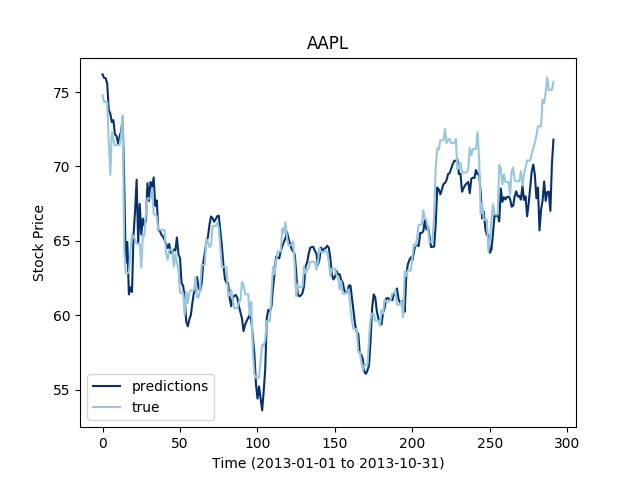
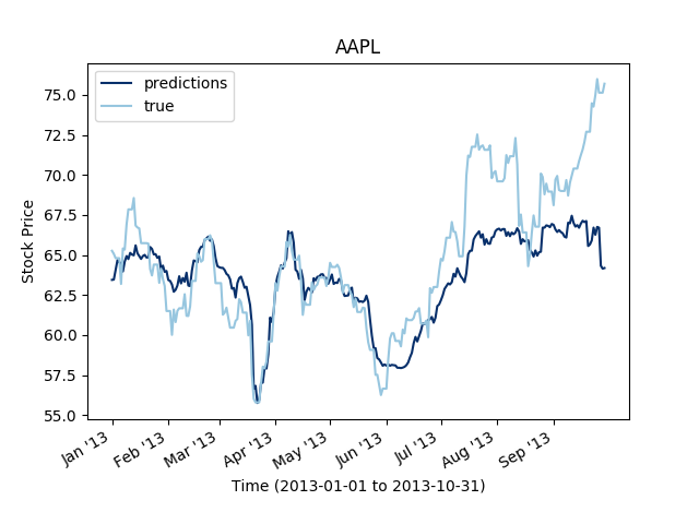
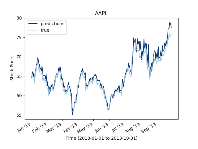
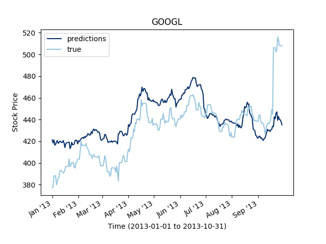
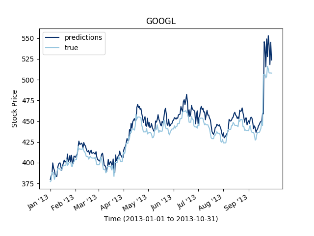
Let's first check what type of prediction errors an LSTM network gets on a simple stock. The training data is the stock price values from 2013-01-01 to 2013-10-31, and the test set is extending this training set to 2014-10-31.
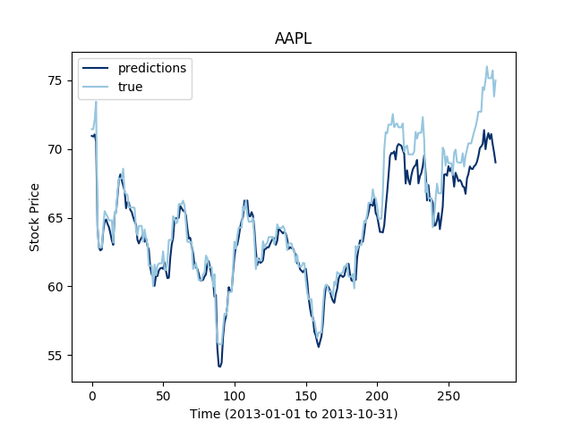
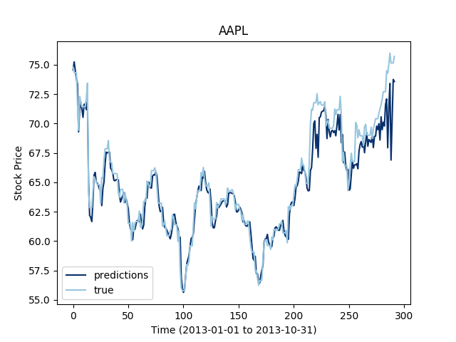
It looks like shuffling the samples may give a slightly lower precision in training, but it give a lower error in testing; shuffling the training samples yields better generalization capacities.
The LSTM are said to work well for multivariate time series, so let's see the extent of this statement on our data set:
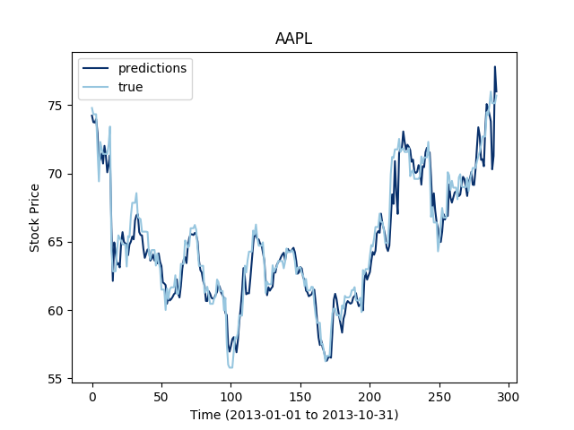
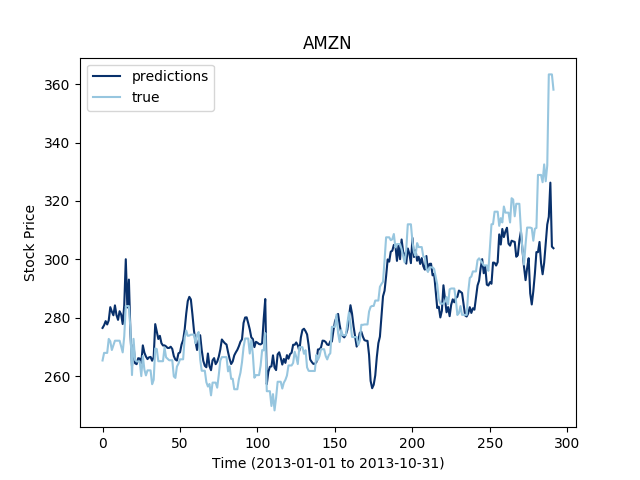
Let's now see how this works for three different stocks at the same time:
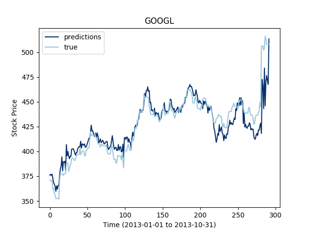
It looks like the more time series we add to the mutiltivariate training, the less the LSTM seems to perform. This makes sense since even through the series are correlated, the construction of the LSTM does not allow the flow of information to focus on one time serie or the other depending on their variations.
Dilated convolution
Another approach that is relevant to predicting time series is the one proposed in the WaveNet paper for 1D signals. While this paper focuses on time sequence generation, the multiscale approach also works for prediction, as seen in the paper Conditional Time Series Forecasting with Convolutional Neural Networks. The idea in this paper is to counter the fact that the -financial- environment is constantly changing - and may render trend extraction a very difficult task over one stock. But there on the other hand is a tremendous amount of data generated in a small time frame; the idea of using different stocks in a same time frame through dilated convolution is hence quite seducing. By using multiple time series as an input to the network, the forecast of one series is conditional to the others, and allows to reduce the effect of noise stochasticity. It is worth noting that the method in the cited paper doesn't perform multivariate prediction.
I experimented something slightly different from the paper mentionned above; a first experiment consisted of using 1D convolutions on different stocks, in order to see the effect of dilated convolutions on each series independently. I decided to test the dilated convolution approach first by using \(n\) stocks in parallel and perform 1D dilated convolution on each stock independently. I used the Pytorch library, with input of dimensions \(n_{batch} \times n_{stocks} \times T \).
from torch import nn


class DilatedNet(nn.Module):
    def __init__(self, num_securities=5, hidden_size=64, dilation=2, T=10):
        """

        :param num_securities: int, number of stocks
        :param hidden_size: int, size of hidden layers
        :param dilation: int, dilation value
        :param T: int, number of look back points
        """
        super(DilatedNet, self).__init__()
        self.dilation = dilation
        self.hidden_size = hidden_size
        # First Layer
        # Input
        self.dilated_conv1 = nn.Conv1d(num_securities, hidden_size, kernel_size=2, dilation=self.dilation)
        self.relu1 = nn.ReLU()

        # Layer 2
        self.dilated_conv2 = nn.Conv1d(hidden_size, hidden_size, kernel_size=1, dilation=self.dilation)
        self.relu2 = nn.ReLU()

        # Layer 3
        self.dilated_conv3 = nn.Conv1d(hidden_size, hidden_size, kernel_size=1, dilation=self.dilation)
        self.relu3 = nn.ReLU()

        # Layer 4
        self.dilated_conv4 = nn.Conv1d(hidden_size, hidden_size, kernel_size=1, dilation=self.dilation)
        self.relu4 = nn.ReLU()

        # Output layer
        self.conv_final = nn.Conv1d(hidden_size, num_securities, kernel_size=1)

        self.T = T

    def forward(self, x):
        """

        :param x: Pytorch Variable, batch_size x n_stocks x T
        :return:
        """

        # First layer
        out = self.dilated_conv1(x)
        out = self.relu1(out)

        # Layer 2:
        out = self.dilated_conv2(out)
        out = self.relu2(out)

        # Layer 3:
        out = self.dilated_conv3(out)
        out = self.relu3(out)

        # Layer 4:
        out = self.dilated_conv4(out)
        out = self.relu4(out)

        # Final layer
        out = self.conv_final(out)
        out = out[:, :, -1]

        return out
Then, in order to take into account the correlation between the series, I used 2D convolutions, but dilated only on the time axis to get this "time multi scale" aspect. Again, I used Pytorch to implement this network, and used inputs of size \(n_{batch} \times 1 \times n_{stocks} \times T\). The \(1\) in the previous dimensions corresponds to the fact that I only used closing prices for estimating stock prices, but other features could easily be added on that dimension in order to take into account other metrics, like the highest/lowest values or the volume.
from torch import nn


class DilatedNet2D(nn.Module):
    def __init__(self, hidden_size=64, dilation=1, T=10):
        """

        :param hidden_size: int, size of hidden layers
        :param dilation: int, dilation value
        :param T: int, number of look back points
        """
        super(DilatedNet2D, self).__init__()
        self.dilation = dilation
        self.hidden_size = hidden_size
        # First Layer
        # Input
        self.dilated_conv1 = nn.Conv2d(1, hidden_size, kernel_size=(1, 2), dilation=(1, self.dilation))
        self.relu1 = nn.ReLU()

        # Layer 2
        self.dilated_conv2 = nn.Conv2d(hidden_size, hidden_size, kernel_size=(1, 2), dilation=(1, self.dilation))
        self.relu2 = nn.ReLU()

        # Layer 3
        self.dilated_conv3 = nn.Conv2d(hidden_size, hidden_size, kernel_size=(1, 2), dilation=(1, self.dilation))
        self.relu3 = nn.ReLU()

        # Layer 4
        self.dilated_conv4 = nn.Conv2d(hidden_size, hidden_size, kernel_size=(1, 2), dilation=(1, self.dilation))
        self.relu4 = nn.ReLU()

        # Output layer
        self.conv_final = nn.Conv2d(hidden_size, 1, kernel_size=(1, 2))

        self.T = T

    def forward(self, x):
        """

        :param x: Pytorch Variable, batch_size x 1 x n_stocks x T
        :return:
        """

        # First layer
        out = self.dilated_conv1(x)
        out = self.relu1(out)

        # Layer 2:
        out = self.dilated_conv2(out)
        out = self.relu2(out)

        # Layer 3:
        out = self.dilated_conv3(out)
        out = self.relu3(out)

        # Layer 4:
        out = self.dilated_conv4(out)
        out = self.relu4(out)

        # Final layer
        out = self.conv_final(out)
        out = out[:, :, :, -1]

        return out

It is notable that the 2D dilated convolutions perform better than the 1D dilated convolutions. It is very likely that the structure is more taken into account in the 2D convolutions and hence, if any correlation exist between the series, the convolution on the stocks dimension will capture some of it.
Conclusion
We have seen a couple of methods for estimating multivariate time series. LSTM seems to work fine for smaller horizon \(T\) than the dilated convolution approach. But overall, 2D convolution seems like a simple and yet efficient method for next day prediction.
Of course, this a quite simple task; predicting time series few days at a time is a challenging issue. This model is also completely "offline"; for real industrial purposes, a more complex and dynamic model would be required.
In the next post, we will see how an attention mechanism can also help predict time series, and generalize this code for multi step time series prediction.
You can leave comments down here, or contact me through the contact form of this blog if you have questions or remarks on this post!