Max Margin Markov Network and Deep Learning

In this post I am going to reformulate the work of my Master Thesis Max Margin Markov Networks and Deep Neural Networks for Stereo Imaging.

The idea of my master Thesis is to mingle deep neural network and graphical model. We know that deep neural networks are great at creating high level features and that Graphical Models are an excellent tool for enforcing structure. In this work, we want to have the best of both approaches. To this end we rely on the Max Margin Markov Network (M3N) framework.

In my Master thesis at Caltech, I proposed a first instantiation of this idea. But it turned out to be very slow and computationally expansive. In this blog post, I revisit the original approach and I propose a equivalent formulation that is much faster.

Graphical Models

Graphical Models have been extensively used in Computer Vision under the form of Markov Random Field, MRF, and Conditional Random Fields, CRF. In this blog, we abusively use the notation MRF for either an MRF or a CRF.

An MRF has a support graph composed of nodes \( \mathcal{V} \) and edges \( \mathcal{E} \). A set of random variables \(x = (x_i)_{i \in \mathcal{V}} \) that all take value in some discrete space \( \mathcal{L} \) represents the configuration of each node. A unary term \( u_i: \mathcal{L} \rightarrow \mathbb{R}\) encodes the cost of each node \( i \in \mathcal{V} \). A pairwise term \( p_{i, j}: \mathcal{L} \times \mathcal{L} \rightarrow \mathbb{R}\) encodes the cost of each edge \( (i,j) \in \mathcal{E} \). The cost of the a given configuration \(x\) is given by: $$ MRF(x) = \sum_{i \in \mathcal{V}} u_i (x_i) + \sum_{(i, j) \in \mathcal{E}} p_{i,j}(x_i, x_j) $$ The configuration of minimum cost of an MRF is called the Maximum A Posteriori configuration: $$ x_{opt} = \underset{x}{\text{argmin}} MRF(x) $$ Computing the MAP is generally an NP-hard problem, so we are only guaranteed to find approximate solutions.

Stereo Matching

In the context of stereo matching, we want to register a reference image, \( I_{ref} \) to a target image \( I_{tar} \). Each pixel of the reference image has along the epipolar line an apparent motion that is called disparity. Hence, we associate a node \( i \) and a discrete random variable \( x_i \) to each pixel of the reference image. The discrete random variable encodes a potential disparity that takes value in \( \mathcal{L} \subset \mathbb{N} \).

The unary terms encodes the likeliness of a potential disparity based on a similarity prior. Hence, they measure how a patch \( P_{ref}(i) \) of the reference image centered around pixel \( i \) is similar to the patch \( P_{tar}(i, x_i) \) of the large image centered around pixel \( i \) translated by disparity \( x_i \). The notion of similarity is encoded by a scoring function \( s \) parametrized by \( \theta \): $$ u_i (x_i; \theta) = s(P_{ref}(i), P_{tar}(i, x_i); \theta) $$ This scoring function can as simple as the sum of absolute difference of the two patches or it can be modeled by a Deep Neural Network as in the Paper of Serguey Szagoruyko .

The pairwise terms enforce a structure prior called regularization based on piecewise smoothness. To this end they penalize the gradient of the disparity. $$ p_{i,j}(x_i, x_j; \lambda, \alpha) = w_{i, j}(I_{ref}; \lambda) \min(|x_i - x_j|, \alpha) $$ The strength of this regularization is modulated by \(w_{i, j}\) so that contours of the disparity align with contours of the reference image: $$ w_{i, j} (I; \lambda) = \lambda_{cst} + \lambda_{grad} \exp (- \lambda_{\sigma^{-1}} |I(i) - I(j)|) $$ Again, we could have use a more complex regularization function where \( w_{i, j} \) will have been modeled as Deep Neural Network.

We now have an MRF that has a set of parameters \(\tau = (\theta, \alpha, \lambda) \). Our goal is to tune automatically those parameters.

What is a Max Margin Markov Network?

Let's assume we are given k-MRFs with associated optimal configurations \(x_{gt}^k \) and common parameters \(\tau \). We want to find the parameters \(\tau \) that will make, ideally, each \(x_{gt}^k \) the Maximum A Posteriori, MAP, solution for \(MRF^k \). Unfortunately since the \( \text{argmin} \) is not differentiable we cannot directly learn the parameters \(\tau \) by minimizing for instance: $$ \begin{align} & \underset{\tau}{\text{minimize}} & \sum_{k} \| x^k_{gt} - \underset{x^k}{\text{argmin}} ~\ MRF^k(x^k; \tau) \| \end{align} $$ However, while \( \text{argmin} \) is not differentiable the operator \( \text{min} \) is differentiable. The Max Margin Markov Network exploits this fact and it attempts to make the energy of ground truth of \( (MRF^k)_k \) to coincide with the MAP energy. To this end, it optimizes: $$ \begin{align} & \underset{\tau}{\text{minimize}} & & R(\tau) + \sum_{k} [ MRF^k (x_{gt}^k ; \tau) - \underset{x_k}{\min} ( {MRF}^k (x^k ; \tau) - \Delta(x_{gt}^k, x^k) )] \end{align} $$ with:

• \(R \) a regularization function of the parameters, optional.
• \(\Delta\) is a margin function that make all solutions different from \(x^k_{gt}\) to have an higher cost.

One can see that the margin function try to enforce the shape of the energy manifold of \( (MRF^k)_k \).

Assuming that we can write \( \underset{x_k}{\min} ( {MRF}^k (x^k ; \tau) - \Delta(x_{gt}^k, x^k) )] \) as a differentiable computational graph, then we can use backpropagation techniques to optimize over \( \tau \). This is were we can derive two approaches.

Master thesis approach

In my Master thesis, I used the dual decomposition solver from Nikos Komodakis to compute a lower bound of \( \underset{x_k}{\min} ( {MRF}^k (x^k ; \tau) - \Delta(x_{gt}^k, x^k) )] \). I embedded this solver directly in the computational graph of the M3N. This resulted in a large computational graph.

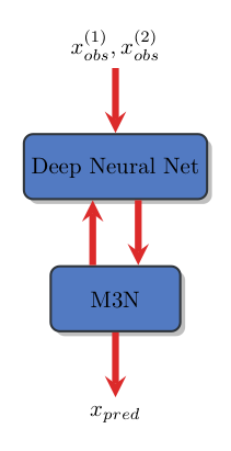
As can be seen in this figure, this naive workflow requires backpropagating the M3N errors through the entire Neural Net and solver. This is very expansive, and also unnecessary...

A more efficient approach

I recently revisited the definition of the computational graph. One can see that in the M3N, there is no need to backpropagate through the variables \( x_{opt}^k \). Let's first introduce: $$ \overline{MRF}^k (x_{opt}^k ; \tau) = \underset{x^k}{\min} {MRF}^k (x^k ; \tau) - \Delta(x_{gt}^k, x^k) $$ We can now simplify the M3N optimization problem as: $$ \begin{align} & \underset{\tau}{\text{minimize}} & & R(\tau) + \sum_k MRF^k (x_{gt}^k ; \tau) - \overline{MRF}^k (x_{opt}^k ; \tau) \end{align} $$

Here is what its associated the computational graph looks like for k=1:

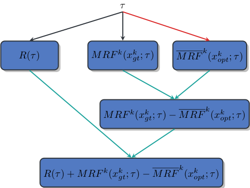
We can observe that \(x^k_{opt}\) is only an input of the computational graph. Hence, we can use any algorithm/implementation for computing: $$ x_{opt}^k = \underset{x^k}{argmin} ~\overline{MRF}^k (x^k ; \tau) $$ Hence, the idea is to alternate between two steps:

• Estimating \( (x^k_{opt})_k \) with a fast non differentiable algorithm (red arrow in previous figure).
• Update the parameters \( \tau \) using the backpropagation (green arrows in previous figure).

I also proceed to change the solver for estimating the MAP. Instead of the lower bound provided by Dual Decomposition, I am using a faster solver (one to two orders of magnitude), Fast-PD, that provides an upper bound of \( \underset{x_k}{\min} ( {MRF}^k (x^k ; \tau) - \Delta(x_{gt}^k, x^k) )] \). However, since we work with an upper bound it's now possible to have: $$ MRF^k (x_{gt}^k ; \tau) \leq \overline{MRF}^k (x_{opt}^k ; \tau) $$ This means that \( x_{gt}^k \) has a lower cost but that the solver was not able to reach it (remember MAP is in general an NP-hard problem). Hence, we simply safeguard the M3N cost as follow: $$ \begin{align} & \underset{\tau}{\text{minimize}} & & R(\tau) + \sum_k \max(MRF^k (x_{gt}^k ; \tau) - \overline{MRF}^k (x_{opt}^k ; \tau), 0) \end{align} $$

Implementation

Thanks to the wonderful library Pytorch, we can model easily this new M3N formulation as a differentiable computational graph. In details we model as a Pytorch module the computation of the energies of \(MRF^k (x_{gt}^k ; \tau) \) and \(\overline{MRF}^k (x_{opt}^k ; \tau) \) along with the regularization cost of \( R(\tau) \).

The variable $x_{opt}$ is only an input of the M3N Pytorch model. One can use a non differentiable algorithm to estimate $x_{opt}$. I used Bruno Conejo's C++ PhD implementation wrapped for Python of Nikos Komodakis' FastPD algorithm.

A few results

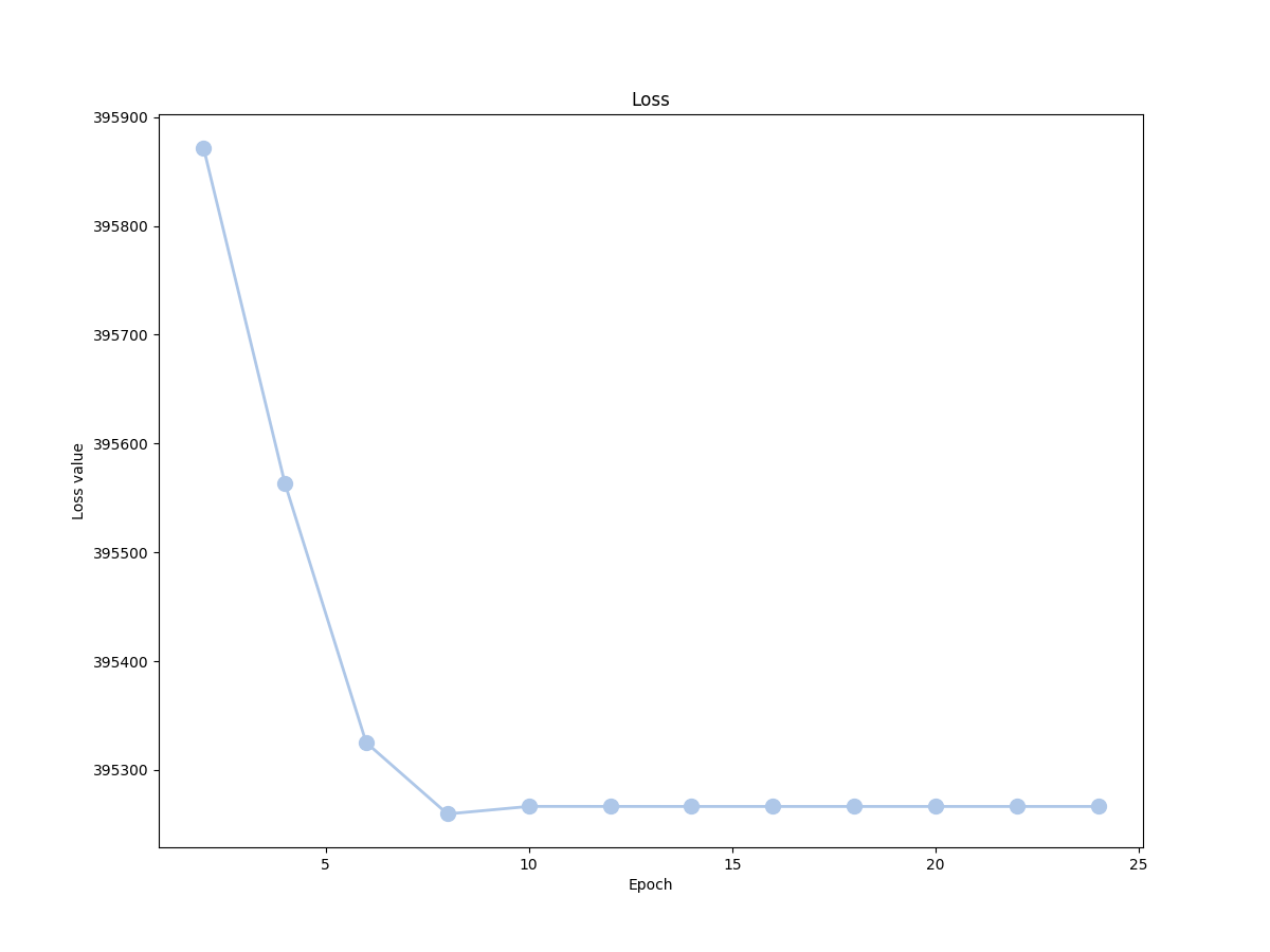
Here is the loss of the network for 20 epochs, on the whole KITTI stereo dataset:

The optimization of the network parameters does converge nicely. For the whole Middlebury 2001 dataset, 10 epochs and 6 pairs of \(432 \times 381 \) images, the experiment takes about 6 minutes (as opposed to a few hours with the previous approach) to run (with CUDA, GTX 1080 Ti, 2 CPU workers).

Here are some results on the Middlebury 2001 dataset:

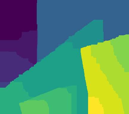
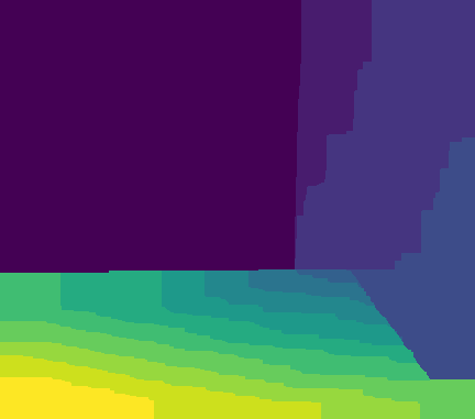
The results are also quite satisfying, considering that our scorer is very simple. In a following blog post, I will explore how this approach performs with a Neural Network for the scorer instead of this similarity function.

You can find the code in its whole here.

You can leave comments down here, or contact me through the contact form of this blog if you have questions or remarks on this post!